Chapter 1: Introduction to Green’s Functions

In recent discussions, we explored the application of Laplace transforms to simplify ordinary differential equations into algebraic forms. If you missed it, you can find the article here:

Using Laplace Transforms in Python to Solve Differential Equations

Today, we will delve into another technique that reduces a differential equation to the evaluation of a single integral—known as "Green's functions."

Consider the following differential equation:

This equation is subject to the initial conditions ( u(0)=0 ) and ( u'(0)=0 ). Previously, we found ( u(t)=cos(4t) ). In this instance, however, we will keep the forcing function general, allowing us to derive solutions applicable to a wide range of differential equations. Our findings will be rooted in the solution of a simpler equation:

Here, ( delta(t) ) denotes the Dirac delta function, which we recently discussed in the article:

A Life Before And After the Dirac Delta Function

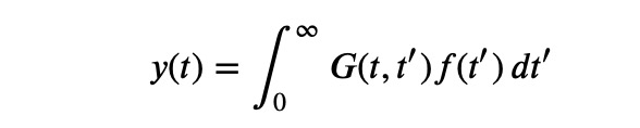
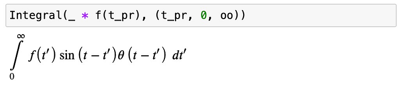
The forcing function in this case represents a single impulse at time ( t_0 ), with zero force at all other times. The concept is that once we determine a solution for this equation, we can "sum up" (integrate) similar solutions for impulses occurring at various times. The solution to a differential equation with a Dirac pulse as the inhomogeneous term is referred to as Green’s function, ( G(t,t_0) ). The summation can be expressed as:

It is straightforward to verify this by substituting this solution back into the differential equation:

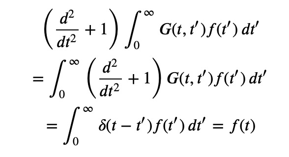
Thus, the integral in the equation indeed satisfies the differential equation. The remaining task is to evaluate the integral for the specific ( f(t) ). However, we first need to ascertain ( G(t,t_0) ), which we will explore next.

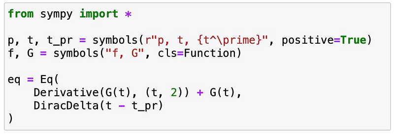
Open a Jupyter notebook and define our symbols and the differential equation:

To tackle this equation, we’ll apply Laplace transforms. We start by transforming the left side:

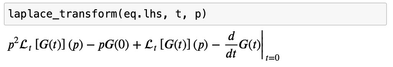
Next, we incorporate the initial conditions:

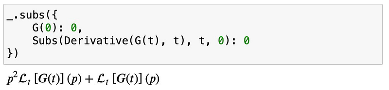
Then, we transform the right side:

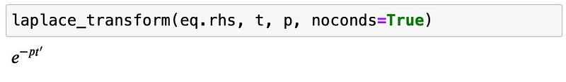
Thus, the transformed equation becomes:

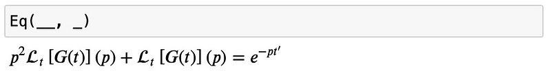
Now, we solve for the Laplace transform of ( G ):

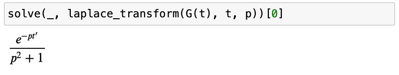
Finally, we revert to the original space:

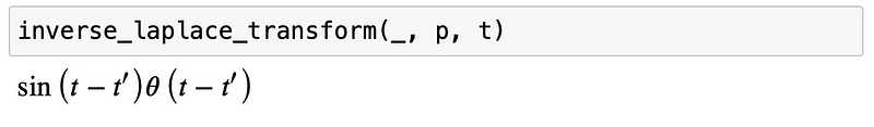
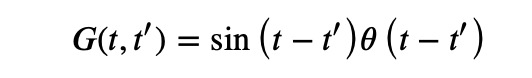
We find that Green’s function for the first differential equation with initial conditions ( u(0)=0 ) and ( u'(0)=0 ) is given by:

This allows us to derive the solution for any forcing function ( f(t) ) by evaluating the integral:

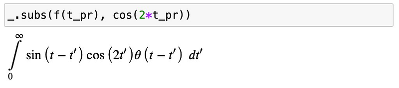
Let’s examine this for the specific case where ( f(t)=cos(2t) ):

Let’s verify whether this indeed satisfies the differential equation:

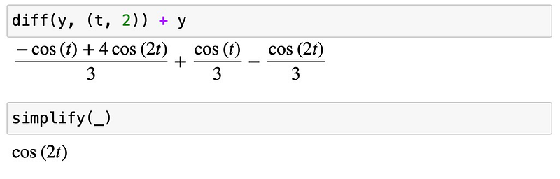
This corresponds to the right side ( f(t) ). So, that checks out. But does it also fulfill the initial conditions?

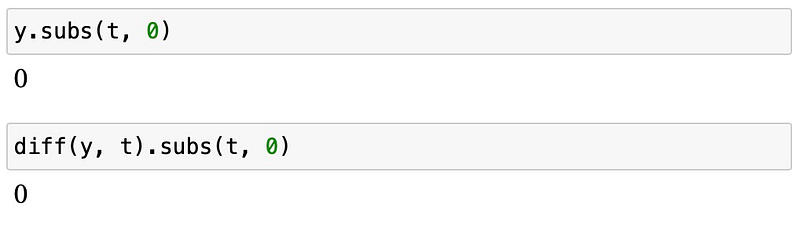
Indeed, it does, and we have reached a conclusion. Different initial conditions or differential equations will yield distinct Green functions. However, once a Green function is identified, the solution becomes accessible, regardless of the applied forcing function.

This brief overview merely scratches the surface of the expansive domain of Green’s functions. A significant portion of quantum field theory revolves around applied Green’s function theory, making it a topic worth exploring further. For those interested in a deeper dive, I highly recommend A. Zee’s excellent book “Quantum Field Theory in a Nutshell” (no, I don’t earn any commission from that link).

Chapter 2: Video Resources for Further Learning

The first video, "Greens Functions for Normies," provides an approachable introduction to the concept of Green's functions.

The second video, "Green's functions: the genius way to solve DEs," offers an insightful perspective on how Green's functions can be utilized to tackle differential equations.