Chapter 1: Introduction to Horner's Method

Recently, I discovered an arithmetic technique known as Horner’s method, which I found quite fascinating. This method is specifically designed for efficiently evaluating polynomials at a specified point by hand. Additionally, it can be employed for polynomial division, finding polynomial roots, or even for partial fraction decomposition. In this article, I will explain how Horner’s method operates and provide a detailed, step-by-step implementation using Python code.

Chapter 2: Understanding the Method

Imagine you have a polynomial and you wish to evaluate it at x=2 manually. Horner’s method relies on the insight that you can always express the polynomial in a more manageable form.

If you're having difficulty grasping this concept, try reading it from right to left!

Next, set up a table where you write the coefficients of the polynomial in the top row. Below the first coefficient, place a zero in the second row. On the left side, note the point where you want to evaluate (x=2 in this case):

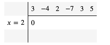
The initial setup of Horner’s method involves repeatedly executing two main steps:

1. If there are entries in the first and second rows of a column, but not in the third, sum the first two entries and write the result in the third row.
2. Multiply the newly obtained value from step 1 by the evaluation point (x=2 here) and place the result in the next available cell of the second row.

For our example, step 1 entails adding 3 and 0, resulting in:

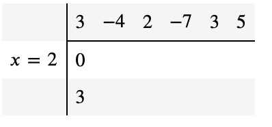
In step 2, you multiply 3 (from the third row) by 2 and write the outcome, 6, next to the 0 in the second row:

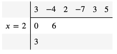
Continue this process, repeating steps 1 and 2, until the table is completely filled:

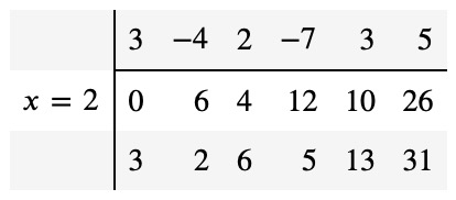
The value of P(x=2) will always be located in the bottom right corner of the table. Moreover, the other values in the third row provide significant insights: they represent the coefficients of the polynomial resulting from dividing P(x) by (x-2).

This illustrates that Horner’s method can also be beneficial for polynomial division.

Chapter 3: Step-by-Step Python Implementation

To begin, install the latest version of the Python package mathcube with the following command:

pip install --upgrade mathcube

Now, launch a Jupyter notebook and make the necessary imports:

Define your polynomial:

And specify the point for evaluation:

Now, initialize Horner’s method:

You can proceed step by step by calling the step() method each time:

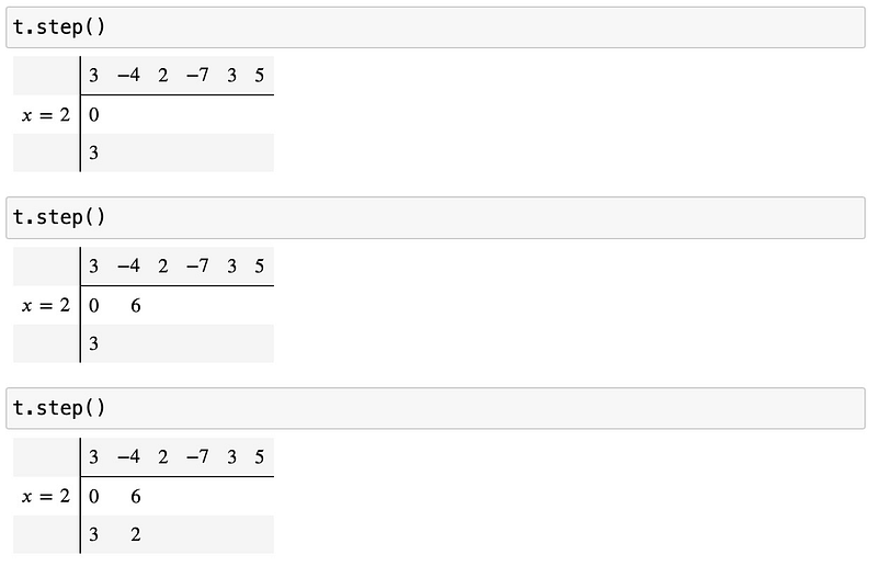
Eventually, you will arrive at the table seen at the end of the previous section. To verify that P(2)=31 is accurate, use SymPy:

And that's a wrap on Horner’s method! We will revisit it soon for additional applications.