Chapter 1: Introduction to Computer Algebra with SymPy

Utilizing computer algebra systems, such as Python's SymPy, can significantly enhance your work efficiency, provided you dedicate ample time to practice. Without sufficient familiarity, one might find themselves sidetracked by the intricacies of the software rather than focusing on the problem at hand. This often leads individuals to revert to traditional methods like paper and pencil after only a brief encounter with these powerful tools. Indeed, the learning curve can be quite challenging, and patience is essential. To assist you in gaining practical experience, I've created this series of articles.

It's important to note that simply reading isn't enough to achieve proficiency. I urge you to start your own Jupyter notebook, engage with the material actively, and experiment with the code.

For today's session, we'll derive Stirling’s formula exclusively using SymPy. This formula serves as an approximation for the factorial function. Specifically,

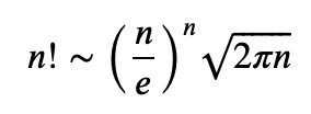
where the symbol “~” indicates that one quantity is asymptotic to another. In simpler terms, the ratio

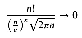
as n approaches infinity. For further insights, refer to my additional article discussing asymptotic expansions. Now, let’s proceed with the derivation using SymPy.

The factorial can be expressed via the Gamma function: n! = Γ(n + 1), where

We will initiate our work in Jupyter by defining n! in terms of the Gamma function.

from sympy.abc import *

from sympy import *

t, n = symbols('t, n', positive=True)

Ii = Integral(t**n * exp(-t), (t, 0, oo))

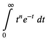
It is helpful to express the integrand using a common base: Ii = Ii.replace(t**n, exp(n*log(t)))

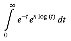
The primary approach involves expanding the logarithm around an appropriate value. However, we currently only have log(t). Therefore, we will make a substitution:

Ii = Ii.transform(t, (n + sqrt(n) * u, u))

It's worth noting that when defining the substitution in SymPy, a tuple is required as the second argument. This is because our substitution rule encompasses two variables, t and u, and SymPy needs to know which variable will serve as the new integration variable. The second entry in the tuple indicates to SymPy that u will be the new variable.

Next, we will refine the logarithm. First, we extract it:

the_log = list(Ii.atoms(log))[0]

The atom function retrieves all relevant heads, in this case, log. To access the log, I convert the set to a list and select the first entry. Within the log's argument, I want to isolate a factor of n:

the_arg = the_log.args[0]

We simplify this further:

n * simplify(the_arg / n)

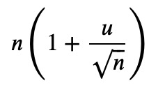
Then, we expand the logarithm:

log(_)

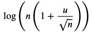
And replace it in our original expression:

Ii2 = Ii.replace(the_log, _)

Since n is large, we can express the logarithm as a power series:

log(1 + u/sqrt(n)).series(u/sqrt(n), 0, 3).removeO()

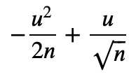
We then substitute this back into our equation:

Ii3 = Ii2.replace(log(1 + u/sqrt(n)), _)

Next, we expand:

Ii3.expand()

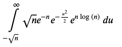
Now, let's instruct SymPy to solve it:

Ii4 = _.doit()

Observe the parentheses in the numerator. As n becomes large, the complementary error function, erfc, will be negligible compared to the leading term. To confirm this, we can expand erfc:

erfc(sqrt(n/2)).series(n, oo)

Indeed, the exponential factor indicates that erfc becomes very small. Thus, we can replace it with zero:

Ii4.replace(erfc, lambda arg: 0)

This version of replace enables the substitution of a function along with its argument, meaning we replace erf(x) with 0 for any x. We can then perform some simplifications:

factor(_)

Finally, we rewrite the second exponential term:

_.replace(exp(n*log(n)), n**n)

And there you have it; we have successfully derived Stirling’s formula using SymPy!

Chapter 2: Enhancing Your Understanding with Video Resources

Explore the fascinating world of symbolic mathematics in Python through this video: "Symbolic Math with Python using SymPy - Talk Python to Me Ep.364." This episode delves into practical applications and tips for mastering SymPy.

For a more detailed tutorial, check out "SymPy Tutorial (2022): For Physicists, Engineers, and Mathematicians." This video covers essential concepts and provides hands-on examples to deepen your understanding of SymPy.